U-Nets for images - Dynamical Transport Book

In what follows we will build out a U-Net architecture for image generation tasks with dynamical transport.¶

The U-Net architecture has its contemporary origins in image-segmentation analysis in medicine (Ronneberger et al. (2015)). A pictorial version of the downsampling and skip connections that are a signature of the U-Net, which allows features to be pushed forward at all scales to the velocity field update, is given in Figure 1.

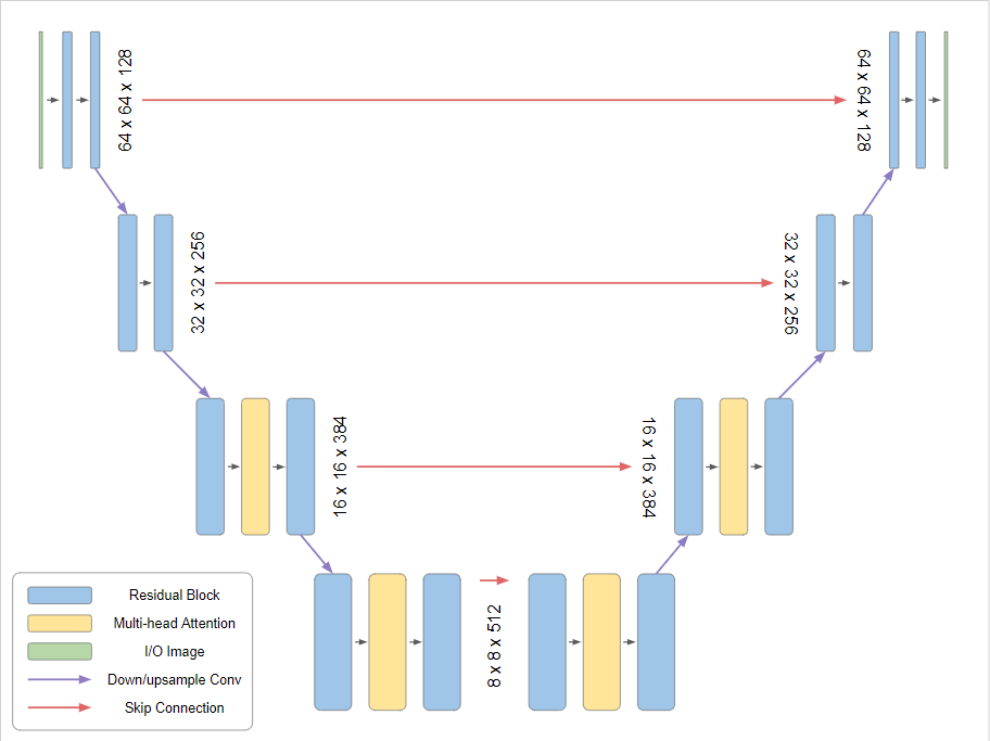
Figure 1:Taken from https://hannibunny.github.io/mlbook/diffusion/denoisingDiffusion.html

In this example we will target modeling the MNIST dataset. An MNIST image is [1, 28, 28] pixels, meaning that each image is a point in $\mathbb R^{28 \times 28}$ . MNIST images are black and white, so the [1] in the image shape specifies that there is only 1 color channel as opposed to RGB.

Note that the U-Net implementation is courtesy of lucidrains on GitHub, whose work is a gift to us all!

In what follows, we’ll describe the pieces of a U-Net so that we can assemble how it represents a vector field or score function in dynamical transport.

import numpy as np
import torch
import matplotlib.pyplot as plt
from torch.func import vmap, jacfwd
from torchvision.datasets import MNIST, CIFAR10


import math

from tqdm import tqdm

device = 'cuda' if torch.cuda.is_available() else 'cpu'
print(torch.cuda.is_available())
print(device)

True
cuda

Let’s first define a number of the previous functions we defined in the previous notebook¶

This includes:

A prior Gaussian distribution
an interpolant class
a loss function
an ODE to integrate as our generative model, as before

In addition we will specify some variables based on the MNIST dataset, as well as some helper functions that help us normalize our images to be in values between [-1,1] and unnormalize them back to [0,1], which is where the image pixel values initially reside.

dset = MNIST 
C = 1  # channels
L = 28 # image H/W

def normalize(x):
    return 2*x -1
def unnormalize(x):
    return (x + 1)/2

Prior¶

class Prior(torch.nn.Module):
    """
    Abstract class for prior distributions of normalizing flows. The interface
    is similar to `torch.distributions.distribution.Distribution`, but batching
    is treated differently. Parameters passed to constructors are never batched,
    but are aware of the target (single) sample shape. The `forward` method then
    accepts just the batch size and produces a batch of samples of the known
    shape.
    """
    def forward(self, batch_size):
        raise NotImplementedError()
    def log_prob(self, x):
        raise NotImplementedError()
    def draw(self, batch_size):
        """Alias of `forward` to allow explicit calls."""
        return self.forward(batch_size)
    
class SimpleNormal(Prior):
    def __init__(self, loc, var, requires_grad = False):
        super().__init__()
        
        if requires_grad:
            loc.requires_grad_()
            var.requires_grad_()
        self.loc = loc
        self.var = var
        self.dist = torch.distributions.normal.Normal(
            torch.flatten(self.loc), torch.flatten(self.var))
        self.shape = loc.shape
        
            
    def log_prob(self, x):
        logp = self.dist.log_prob(x.reshape(x.shape[0], -1))
        return torch.sum(logp, dim=1)
    def forward(self, batch_size):
        x = self.dist.sample((batch_size,))
        return torch.reshape(x, (-1,) + self.shape)
    
    def rsample(self, batch_size):
        x = self.dist.rsample((batch_size,))
        return torch.reshape(x, (-1,) + self.shape)

We make are our base distirbution using the MNIST channel count and image size.

base = SimpleNormal(torch.zeros((C,L,L)), torch.ones(C,L,L))

Loss function¶

In the loss function we now include image classes, which will be fed to our velocity field for conditional modeling

def _single_loss(b, interpolant, x0, x1, t, classes):
    """
    Interpolant loss function for a single datapoint of (x0, x1, t).
    """
    It          = interpolant._single_xt(x0, x1, t)
    dtIt        = interpolant._single_dtxt(x0, x1, t)
    
    btx   = b._single_forward(It, t, classes)
    loss = ((btx - dtIt)**2).sum()

    return loss

loss_fn = vmap(_single_loss, 
               in_dims=(None, None, 0, 0, 0, 0), 
               out_dims = (0), 
               randomness='different')

Interpolant¶

We again set up our interpolant just as before

class Interpolant:
    def alpha(self, t):
        return 1.0 - t
    
    def dotalpha(self, t):
        return -1.0
    
    def beta(self, t):
        return t
    
    def dotbeta(self, t):
        return 1.0
    
    def _single_xt(self, x0, x1, t):
        return self.alpha(t)*x0 + self.beta(t)*x1
    
    def _single_dtxt(self, x0, x1, t):
        return self.dotalpha(t)*x0 + self.dotbeta(t)*x1
    
    def xt(self, x0, x1, t):
        return vmap(self._single_xt, in_dims=(0, 0, 0))(x0,x1,t)
    
    def dtxt(self, x0, x1, t):
        return vmap(self._single_dtxt, in_dims=(0, 0, 0))(x0,x1,t)
    
interpolant = Interpolant()

ODE integrator¶

And finally the ODE.

class ODE:
    def __init__(self, b, interpolant, n_step):
        
        self.b           = b
        self.interpolant = interpolant
        self.n_step      = n_step
        self.ts          = torch.linspace(0.0,1.0, n_step + 1).to(device)
        self.dt          = self.ts[1] - self.ts[0]
    
    
    
    def step(self, x, t, c):
        return x + self.b(x, t, c)*self.dt 
    
    def solve(self, x_init, classes):
        
        bs = x_init.shape[0]
        xs = torch.zeros((self.n_step, *x_init.shape))
        x = x_init
        
        with torch.no_grad():
            for i,t in enumerate(self.ts[:-1]):
                t = t.repeat(len(x))
                x = self.step(x,t, classes)
                xs[i] = x
            return xs

Now, we turn to our U-Net.¶

The purpose of the U-Net is to share information across scales and to push forward a the difference of the current $x_t$ to what the new $x_{t+h}$ might be in a ODE integrator (maybe one nice way of many to think about it.)

As such, our model will have a number of downsampling features, whose representations are saved, as well as a bunch of upsampling features, upon which the downsampling features are added (to propagate forward information).

First, we import some helper functions, no need to worry about these.¶

from functools import partial
from collections import namedtuple

import torch
from torch import nn, einsum
import torch.nn.functional as F

from einops import rearrange





# COPIED FROM THE AMAZING LUCIDRAINS https://github.com/lucidrains/denoising-diffusion-pytorch/blob/main/denoising_diffusion_pytorch/guided_diffusion.py


# helpers functions

def exists(x):
    return x is not None

def default(val, d):
    if exists(val):
        return val
    return d() if callable(d) else d

def identity(t, *args, **kwargs):
    return t

def cycle(dl):
    while True:
        for data in dl:
            yield data

def has_int_squareroot(num):
    return (math.sqrt(num) ** 2) == num

def num_to_groups(num, divisor):
    groups = num // divisor
    remainder = num % divisor
    arr = [divisor] * groups
    if remainder > 0:
        arr.append(remainder)
    return arr

def convert_image_to_fn(img_type, image):
    if image.mode != img_type:
        return image.convert(img_type)
    return image

Downsampling and Upsampling¶

The first thing we do in the U-Net is we apply a convolution to downsample our image and add a number of new feature channels. Later on, we will perform an inverse-like operation, which uses another convolution to upsample the image back to a new resolution and smaller set of features.

def Downsample(dim, dim_out = None):
    return nn.Conv2d(dim, default(dim_out, dim), 4, 2, 1)

def Upsample(dim, dim_out = None):
    return nn.Sequential(
        nn.Upsample(scale_factor = 2, mode = 'nearest'),
        nn.Conv2d(dim, default(dim_out, dim), 3, padding = 1)
    )

Time and class embeddings¶

Because our velocity field will receive a time value as well as potentially a class label, we want to embed those into a high dimensional, richer feature so that this information is properly utilized in the network.

We could either use some sort of sinuisoidal, periodic embedding, or we could choose to add learned features to this:

class SinusoidalPosEmb(nn.Module):
    def __init__(self, dim):
        super().__init__()
        self.dim = dim

    def forward(self, x):
        device = x.device
        half_dim = self.dim // 2
        emb = math.log(10000) / (half_dim - 1)
        emb = torch.exp(torch.arange(half_dim, device=device) * -emb)
        emb = x[:, None] * emb[None, :]
        emb = torch.cat((emb.sin(), emb.cos()), dim=-1)
        return emb
    
    
class RandomOrLearnedSinusoidalPosEmb(nn.Module):
    """ following @crowsonkb 's lead with random (learned optional) sinusoidal pos emb """
    """ https://github.com/crowsonkb/v-diffusion-jax/blob/master/diffusion/models/danbooru_128.py#L8 """

    def __init__(self, dim, is_random = False, unet_fourier_scale = 0.02):
        super().__init__()
        assert (dim % 2) == 0
        half_dim = dim // 2
        init_weights = torch.normal(0.0, unet_fourier_scale, size=(half_dim,))
        self.weights = nn.Parameter(init_weights, requires_grad = not is_random)

    def forward(self, x):
        x = rearrange(x, 'b -> b 1')
        freqs = x * rearrange(self.weights, 'd -> 1 d') * 2 * math.pi
        fouriered = torch.cat((freqs.sin(), freqs.cos()), dim = -1)
        fouriered = torch.cat((x, fouriered), dim = -1)
        return fouriered

Residual Networks and Attention at each block¶

Along the down sampling and upsampling blocks, a residual network type layer is instantiated that, using time and class embeddings, adds new processed features to the existing input (this is the “residual type feature”).

Usually at each downsampling stage, we do this twice, followed by an action of linear attention, which is a cheaper version of attention that doesn’t attend on the whole image but allows to aggregate spatial information in the image.

A variety of normalization techniques to normalize the values are applied at this point too.

class Residual(nn.Module):
    """Class that, given some function producing features, adds these features to existing input"""
    def __init__(self, fn):
        super().__init__()
        self.fn = fn

    def forward(self, x, *args, **kwargs):
        return self.fn(x, *args, **kwargs) + x

    
### used to normalize features
class RMSNorm(nn.Module):
    def __init__(self, dim):
        super().__init__()
        self.g = nn.Parameter(torch.ones(1, dim, 1, 1))

    def forward(self, x):
        return F.normalize(x, dim = 1) * self.g * (x.shape[1] ** 0.5)

class PreNorm(nn.Module):
    def __init__(self, dim, fn):
        super().__init__()
        self.fn = fn
        self.norm = RMSNorm(dim)

    def forward(self, x):
        x = self.norm(x)
        return self.fn(x)
    
    
    
class LinearAttention(nn.Module):
    """Has O(N) complexity rather than O(N^2) b/c doesn't compute one interaction of the queries and keys q* k^T."""
    def __init__(self, dim, heads = 4, dim_head = 32):
        super().__init__()
        self.scale = dim_head ** -0.5
        self.heads = heads
        hidden_dim = dim_head * heads
        self.to_qkv = nn.Conv2d(dim, hidden_dim * 3, 1, bias = False)

        self.to_out = nn.Sequential(
            nn.Conv2d(hidden_dim, dim, 1),
            RMSNorm(dim)
        )

    def forward(self, x):
        b, c, h, w = x.shape
        qkv = self.to_qkv(x).chunk(3, dim = 1)
        q, k, v = map(lambda t: rearrange(t, 'b (h c) x y -> b h c (x y)', h = self.heads), qkv)

        q = q.softmax(dim = -2)
        k = k.softmax(dim = -1)

        q = q * self.scale

        context = torch.einsum('b h d n, b h e n -> b h d e', k, v)

        out = torch.einsum('b h d e, b h d n -> b h e n', context, q)
        out = rearrange(out, 'b h c (x y) -> b (h c) x y', h = self.heads, x = h, y = w)
        return self.to_out(out)

class Attention(nn.Module):
    def __init__(self, dim, heads = 4, dim_head = 32):
        super().__init__()
        self.scale = dim_head ** -0.5
        self.heads = heads
        hidden_dim = dim_head * heads

        self.to_qkv = nn.Conv2d(dim, hidden_dim * 3, 1, bias = False)
        self.to_out = nn.Conv2d(hidden_dim, dim, 1)

    def forward(self, x):
        b, c, h, w = x.shape
        qkv = self.to_qkv(x).chunk(3, dim = 1)
        q, k, v = map(lambda t: rearrange(t, 'b (h c) x y -> b h c (x y)', h = self.heads), qkv)

        q = q * self.scale

        sim = einsum('b h d i, b h d j -> b h i j', q, k)
        attn = sim.softmax(dim = -1)
        out = einsum('b h i j, b h d j -> b h i d', attn, v)

        out = rearrange(out, 'b h (x y) d -> b (h d) x y', x = h, y = w)
        return self.to_out(out)

Next we define the ResNet block¶

Here is where the Block and ResNet block classes are defined. The blocks provide convolutions on the current features, and can scale and shift the values based on the time and class embeddings.

These blocks are used in the ResNet block, on which the final features are added to the original input in a “residual way” to help with gradient propagation.

# building block modules

class Block(nn.Module):
    def __init__(self, dim, dim_out, groups = 8):
        super().__init__()
        self.proj = nn.Conv2d(dim, dim_out, 3, padding = 1)
        self.norm = nn.GroupNorm(groups, dim_out)
        self.act = nn.SiLU()

    def forward(self, x, scale_shift = None):
        x = self.proj(x)
        x = self.norm(x)

        if exists(scale_shift):
            scale, shift = scale_shift
            x = x * (scale + 1) + shift

        x = self.act(x)
        return x

class ResnetBlock(nn.Module):
    def __init__(self, dim, dim_out, *, time_emb_dim, classes_emb_dim = None, groups = 8):
        super().__init__()

        assert time_emb_dim is not None
        assert time_emb_dim > 0

        int_time_emb_dim = int(time_emb_dim) 
        int_classes_emb_dim = int(classes_emb_dim) if classes_emb_dim is not None else 0
        int_both = int_time_emb_dim + int_classes_emb_dim

        self.mlp = nn.Sequential(
            nn.SiLU(),
            nn.Linear(int_both, dim_out * 2)
        ) 

        self.block1 = Block(dim, dim_out, groups = groups)
        self.block2 = Block(dim_out, dim_out, groups = groups)
        self.res_conv = nn.Conv2d(dim, dim_out, 1) if dim != dim_out else nn.Identity()

    def forward(self, x, time_emb = None, class_emb = None):

        scale_shift = None
        if exists(self.mlp) and (exists(time_emb) or exists(class_emb)):
            cond_emb = tuple(filter(exists, (time_emb, class_emb)))
            cond_emb = torch.cat(cond_emb, dim = -1)
            cond_emb = self.mlp(cond_emb)
            cond_emb = rearrange(cond_emb, 'b c -> b c 1 1')
            scale_shift = cond_emb.chunk(2, dim = 1)

        h = self.block1(x, scale_shift = scale_shift)

        h = self.block2(h)

        return h + self.res_conv(x)

Assembling the model as Unet¶

These tools are used to construct the up and down sampling paths. In the forward pass, we move through these up-sampling and downsampling paths, where the downsampling features are stored in a list h=[] that are passed forward as skip connections on the upsampling pass.

Full attention is only used at the smallest image size for complexity reasons.



class Unet(nn.Module):
    def __init__(
        self,
        num_classes,
        in_channels,
        out_channels,
        dim = 128,
        dim_mults = (1, 2, 2, 2), #,(1, 2, 4, 8),
        resnet_block_groups = 8,
        learned_sinusoidal_cond = True,
        random_fourier_features = False,
        learned_sinusoidal_dim = 32,
        attn_dim_head = 64,
        attn_heads = 4,
        use_classes = True,
        unet_fourier_scale = .02
    ):

        super().__init__()

        # determine dimensions
        
        self.unet_fourier_scale = unet_fourier_scale

        self.use_classes = use_classes

        self.in_channels = in_channels
        input_channels = in_channels

        init_dim = dim
        self.init_conv = nn.Conv2d(input_channels, init_dim, 7, padding = 3)

        dims = [init_dim, *map(lambda m: dim * m, dim_mults)]
        in_out = list(zip(dims[:-1], dims[1:]))

        block_klass = partial(ResnetBlock, groups = resnet_block_groups)

        # time embeddings

        time_dim = dim * 4

        self.random_or_learned_sinusoidal_cond = learned_sinusoidal_cond or random_fourier_features

        if self.random_or_learned_sinusoidal_cond:
            sinu_pos_emb = RandomOrLearnedSinusoidalPosEmb(learned_sinusoidal_dim, random_fourier_features, self.unet_fourier_scale)
            fourier_dim = learned_sinusoidal_dim + 1 ## changed from 1 to 2 for second time
        else:
            sinu_pos_emb = SinusoidalPosEmb(dim)
            fourier_dim = dim
        
        
        self.time_mlp = nn.Sequential(
            sinu_pos_emb,
            nn.Linear(fourier_dim, time_dim),
            nn.GELU(),
            nn.Linear(time_dim, time_dim)
        )

        # class embeddings

        if self.use_classes:
            print("USING CLASSES IN UNET")

            self.classes_emb = nn.Embedding(num_classes, dim)

            classes_dim = dim * 4

            self.classes_mlp = nn.Sequential(
                nn.Linear(dim, classes_dim),
                nn.GELU(),
                nn.Linear(classes_dim, classes_dim)
            )
        else:
            print("NOT USING CLASSES IN UNET")
            classes_dim = None

        # layers

        self.downs = nn.ModuleList([])
        self.ups = nn.ModuleList([])
        num_resolutions = len(in_out)

        for ind, (dim_in, dim_out) in enumerate(in_out):
            is_last = ind >= (num_resolutions - 1)

            self.downs.append(nn.ModuleList([
                block_klass(dim_in, dim_in, time_emb_dim = time_dim, classes_emb_dim = classes_dim),
                block_klass(dim_in, dim_in, time_emb_dim = time_dim, classes_emb_dim = classes_dim),
                Residual(PreNorm(dim_in, LinearAttention(dim_in))),
                Downsample(dim_in, dim_out) if not is_last else nn.Conv2d(dim_in, dim_out, 3, padding = 1)
            ]))

        mid_dim = dims[-1]
        self.mid_block1 = block_klass(mid_dim, mid_dim, time_emb_dim = time_dim, classes_emb_dim = classes_dim)
        self.mid_attn = Residual(PreNorm(mid_dim, Attention(mid_dim, dim_head = attn_dim_head, heads = attn_heads)))
        self.mid_block2 = block_klass(mid_dim, mid_dim, time_emb_dim = time_dim, classes_emb_dim = classes_dim)

        for ind, (dim_in, dim_out) in enumerate(reversed(in_out)):
            is_last = ind == (len(in_out) - 1)

            self.ups.append(nn.ModuleList([
                block_klass(dim_out + dim_in, dim_out, time_emb_dim = time_dim, classes_emb_dim = classes_dim),
                block_klass(dim_out + dim_in, dim_out, time_emb_dim = time_dim, classes_emb_dim = classes_dim),
                Residual(PreNorm(dim_out, LinearAttention(dim_out))),
                Upsample(dim_out, dim_in) if not is_last else  nn.Conv2d(dim_out, dim_in, 3, padding = 1)
            ]))

        self.out_channels = out_channels

        self.final_res_block = block_klass(dim * 2, dim, time_emb_dim = time_dim, classes_emb_dim = classes_dim)
        self.final_conv = nn.Conv2d(dim, self.out_channels, 1)



    def forward(self, x, time, classes = None):

        batch, device = x.shape[0], x.device

 
        if classes is not None:
            if len(classes.shape) == 0:
                classes = rearrange(classes, ' -> 1')
            classes_emb = self.classes_emb(classes)
            c = self.classes_mlp(classes_emb)
        else:

            c = None

        x = self.init_conv(x)
        r = x.clone()
        
        t = self.time_mlp(time)

        h = []

        for block1, block2, attn, downsample in self.downs:
            x = block1(x, t, c)
            h.append(x)

            x = block2(x, t, c)
            x = attn(x)
            h.append(x)

            x = downsample(x)

        x = self.mid_block1(x, t, c)
        x = self.mid_attn(x)
        x = self.mid_block2(x, t, c)

        for block1, block2, attn, upsample in self.ups:
            x = torch.cat((x, h.pop()), dim = 1)
            x = block1(x, t, c)

            x = torch.cat((x, h.pop()), dim = 1)
            x = block2(x, t, c)
            x = attn(x)

            x = upsample(x)

        x = torch.cat((x, r), dim = 1)

        x = self.final_res_block(x, t, c)
        return self.final_conv(x)

Make our U-Net model¶

Below we specify the input arguments to setting up the U-Net

##
num_classes             = 10        ## number of digits
in_channels             = 1         ## black and white image
out_channels            = 1         ## black and white image
dim                     = 64        ## feature dimension (number of channels after first convolution)
dim_mults               = (1, 2, 2) ## a tuple or list of multipliers that define how the dimension changes at each U-Net level
resnet_block_groups     = 8         ## the number of groups in the group normalization layers within each ResNet block (configures GroupNorm layers)
learned_sinusoidal_cond = False     ## whether or not to use learned sinuisoidal embeddings at each time step or to just use (if true, use RandomOrLearnedSinusoidalPosEmb, otherwise standard SinusoidalPosEmb)
learned_sinusoidal_dim  = 32        ## dimension of the feature space of the learned sinuisoidal embedding if using learned
attn_heads              = 8         ## The number of attention heads to use in the attention and linear attention blocks


net = Unet( 
    num_classes = num_classes,
    in_channels = in_channels,
    out_channels = out_channels,
    dim = dim,
    dim_mults = dim_mults, 
    resnet_block_groups = resnet_block_groups,
    learned_sinusoidal_cond = learned_sinusoidal_cond,
    learned_sinusoidal_dim = learned_sinusoidal_dim,
    attn_heads = attn_heads,
    use_classes = True
) 

### test that the U-Net evaluates
bs = 10
x = torch.randn((bs, C, L, L))
t = torch.rand(bs)
c = torch.randint(low=0, high = 9, size=(bs,))
net(x,t,c).shape

USING CLASSES IN UNET

torch.Size([10, 1, 28, 28])

Wrap it in a Velocity class to streamline loss function¶

We want to have a “single_forward” function call that makes vmapping in the loss easier, so we set that up with a Velocity class:

class Velocity(torch.nn.Module):
    def __init__(self, net):
        super(Velocity, self).__init__()
        
        self.net = net

    def _single_forward(self, x, t, classes):  
        x       = x.unsqueeze(0)
        t       = t.unsqueeze(0)
        classes = classes.unsqueeze(0)
        out = self.net(x, t, classes).squeeze()
        out = out.unsqueeze(0) ### necessary for MNIST which only has one channel
        return out
    
    def forward(self, x,  t, classes):
        return vmap(self._single_forward, in_dims=(0,0,0), out_dims=(0), randomness='different')(x, t, classes)

Load the MNIST dataset¶

In what follows we load the MNIST dataset from PyTorch. This is easy to do from existing functions. We will import a number of tools from torchvision, which is a software package attached to torch that helps with computer vision related tasks, including visualizing images.

import torchvision
from torchvision.datasets import MNIST, CIFAR10
from torchvision import transforms
from torch.utils.data import DataLoader



# Define a transform to normalize the data
transform = transforms.Compose([
    transforms.ToTensor(),
])

trainset   = dset('~/.pytorch/' + str(dset) + '_data/', download=True, train=True, transform=transform)
dataloader = DataLoader(trainset, batch_size=bs, shuffle=True)


iterator = iter(dataloader)

Train step¶

def train_step_b(b, interpolant, base, opt, sched, iterator):

    xs = next(iterator)
    x1s, classes = xs[0], xs[1]
    

    x1s = normalize(x1s).to(device)  ## maps data to [-1,1], as generative modeling is easier there
    classes = classes.to(device)
    N   = x1s.shape[0]
    x0s = base(N).to(x1s)
    ts  = torch.rand(N).to(x1s)

    loss_val = loss_fn(b, 
                       interpolant, 
                       x0s, 
                       x1s, 
                       ts, 
                       classes
                       ).mean()
    
    loss_val.backward()
    opt.step()
    sched.step()
    
    
    max_norm = 50
    torch.nn.utils.clip_grad_norm_(b.parameters(), max_norm)  # Clip gradients to prevent explosion
    opt.step()
    sched.step()
    opt.zero_grad()
    
    res = {
            'loss': loss_val.detach().cpu(),
        }
    return res

Training parameters¶

Set the training parameters for the training loop and set up the optimizers

n_opt     = 5000
bs        = 100
plot_freq = 500
n_step    = 25

b = Velocity(net).to(device)
lr = 1e-3 ## learning rate
opt = torch.optim.Adam([
    {'params': b.parameters(), 'lr': lr} ])
sched = torch.optim.lr_scheduler.StepLR(opt, step_size=1000, gamma=0.8)

Train!¶

We’ll plot some samples as we go

losses_b = []

j = 0
# pbar = tqdm(range(n_opt))
pbar = tqdm(range(len(losses_b), n_opt))
for i in pbar:
    # print(i)
    res = train_step_b(b, interpolant, base, opt, sched, iterator)
    loss = res['loss'].detach().numpy().mean()
    losses_b.append(loss)
    pbar.set_description(f'Loss: {loss:.4f}')
    if i % plot_freq == 0:
        
        # sample the map using n_steps
        ode    = ODE(b, interpolant, n_step= 80)
        bs_samp = 16
        x_init = base(bs_samp).to(device)
        classes = torch.randint(0,9, size=(bs_samp,)).to(device)

        xfs    = ode.solve(x_init, classes).to(device)
        x1s = xfs[-1].detach().cpu()#.numpy()
        grid = torchvision.utils.make_grid(unnormalize(x1s.detach()), nrow=4, normalize=False)  # Adjust nrow as needed

        # Show images
        fig = plt.figure(figsize = (10,5))
        plt.imshow(grid.permute(1,2,0).detach().cpu())
        plt.show()

Loss: 1255.2626:   0%|          | 0/5000 [00:00<?, ?it/s]Clipping input data to the valid range for imshow with RGB data ([0..1] for floats or [0..255] for integers).

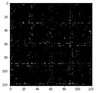
Loss: 264.1428:  10%|█         | 500/5000 [00:26<03:45, 19.99it/s]  Clipping input data to the valid range for imshow with RGB data ([0..1] for floats or [0..255] for integers).

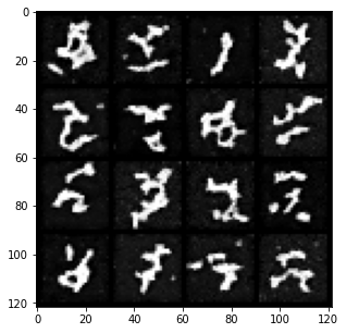
Loss: 165.3679:  20%|█▉        | 999/5000 [00:52<03:18, 20.17it/s]Clipping input data to the valid range for imshow with RGB data ([0..1] for floats or [0..255] for integers).

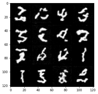
Loss: 197.1455:  30%|███       | 1500/5000 [01:18<02:51, 20.37it/s]Clipping input data to the valid range for imshow with RGB data ([0..1] for floats or [0..255] for integers).

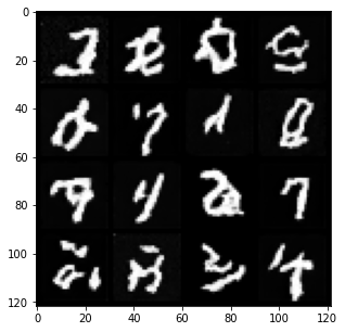
Loss: 158.3646:  40%|████      | 2000/5000 [01:44<02:43, 18.32it/s]Clipping input data to the valid range for imshow with RGB data ([0..1] for floats or [0..255] for integers).

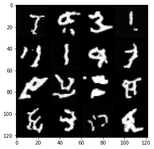
Loss: 173.7022:  50%|████▉     | 2498/5000 [02:11<02:04, 20.13it/s]Clipping input data to the valid range for imshow with RGB data ([0..1] for floats or [0..255] for integers).

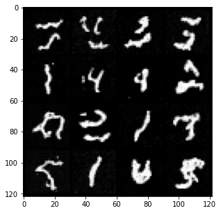
Loss: 140.2697:  60%|█████▉    | 2999/5000 [02:38<01:38, 20.23it/s]Clipping input data to the valid range for imshow with RGB data ([0..1] for floats or [0..255] for integers).

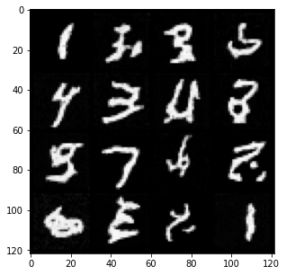
Loss: 167.8616:  70%|██████▉   | 3499/5000 [03:04<01:15, 20.01it/s]Clipping input data to the valid range for imshow with RGB data ([0..1] for floats or [0..255] for integers).

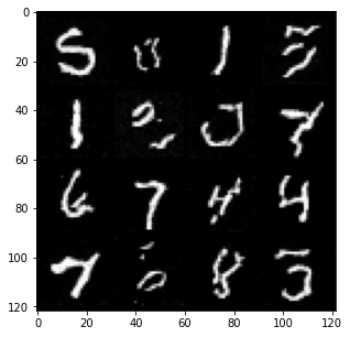
Loss: 162.0897:  80%|███████▉  | 3999/5000 [03:30<00:49, 20.07it/s]Clipping input data to the valid range for imshow with RGB data ([0..1] for floats or [0..255] for integers).

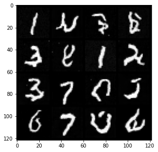
Loss: 152.8408:  90%|████████▉ | 4499/5000 [03:56<00:24, 20.04it/s]Clipping input data to the valid range for imshow with RGB data ([0..1] for floats or [0..255] for integers).

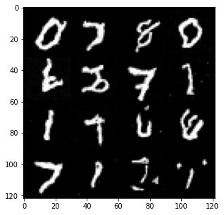
Loss: 122.4328: 100%|██████████| 5000/5000 [04:23<00:00, 18.99it/s]

Plot the losses¶

plt.plot(losses_b)
plt.yscale('log')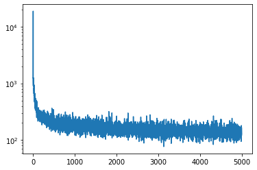

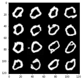
# classes = torch.randint(0,9, size=(bs_samp,))
x_init = base(bs_samp).to(device)
classes = torch.tensor(0).int().repeat(bs_samp).to(device)
xfs    = ode.solve(x_init, classes).to(device)
x1s = xfs[-1].detach().cpu()#.numpy()
grid = torchvision.utils.make_grid(unnormalize(x1s.detach()), nrow=4, normalize=False)  # Adjust nrow as needed

# Show images
fig = plt.figure(figsize = (10,5))
plt.imshow(grid.permute(1,2,0).detach().cpu())
plt.show()

Clipping input data to the valid range for imshow with RGB data ([0..1] for floats or [0..255] for integers).

References¶

Ronneberger, O., Fischer, P., & Brox, T. (2015). U-Net: Convolutional Networks for Biomedical Image Segmentation. https://arxiv.org/abs/1505.04597

Dynamical Transport Book

Deriving and building an image generative model from scratch

Dynamical Transport Book

Appendix