Deriving and building an image generative model from scratch

Figure 1:A sample from OpenAI’s text-to-video model Sora showing a surreal and expedited lifecycle of a flower.

Hello! This self-contained notebook will derive how to arrive at a skeleton of contemporary continuous-variable generative models from scratch.

You are certain to have interacted in some form or another with some artificially generated content in your daily life. It may be some you made yourself, for creative purposes like the the growing flower depicted in the video above courtesy of OpenAI’s Sora model, or one you came across online (for better or for worse). Below we will go through a pedagogical tour through some of the mathematics behind these models and a step-by-step procedure of how to build them ourselves.

Agenda¶

We’ll start with stating what the learning problem is -- finding a map $T: \mathbb R^d \rightarrow \mathbb R^d$ between to probability densities, and describe some ways people have thought about constructing it in the past.
Because we will suggest a continuous-time mapping between the two distributions, we’ll lay out some of the mathematics underpinning this, separate from any generative models or neural networks. This will give us an intuition about ODEs and SDEs.
Then we’ll explain how these ideas can be used to build generative models. From there, we’ll build a toy generative model to complete the picture. Then, learn about more expressive neural networks used to in large scale image generation technologies built on these methods.

Dynamical Transport as a generative model¶

Let’s state plainly what our goals are: given some data $x_1 \in \mathbb R^d$ that are sampled according to some unknown probability density $\rho_1$ , learn a model $\hat \rho_1$ for this distribution that allows us to draw new samples from it. A salient way to do this is to learn a map $T$ that connects points $x_0$ from some simple distribution with density $\rho_0$ to points $x_1 = T(x_0)$ . The characteristics of this map will thereby also tell us how $\rho_0$ is adapted into some $\rho_1$ .

The predominant way to formulate this problem in recent literature is to think about a continuous adaptation of $\rho_0$ into $\rho_1$ , which we will call $\rho_t$ indexed by a some time variable $t \in [0, 1]$ . The paradigmatic method for doing this is score-based/denoising diffusion (Ho et al. (2020), Song et al. (2020)), in which independent Gaussian noise is iteratively denoised into an image. On a per-sample basis, generating an image of a flower, say, might look like what is depicted in Figure 2.

Figure 2:A continuous deformation of Gaussian noise into an image of a flower.

In what follows we’ll analyze the equations that the density $\rho_t$ and the sample $x_t$ must obey to properly perform this generation. Along the way, we’ll derive some algorithms for learning models of the coefficients in the resulting equations that will give us our generative model.

Transporting densities and their samples: Continuity equation and characteristic curves¶

However we adapt $\rho_t$ into $\rho_1$ , we want to ensure that it remains a valid probability density, meaning that the evolution of $\rho_t$ conserves probability mass. Let’s think about how that might come about by imagining probability mass as a fluid, in a simple 3-dimensional example. Assume we have an incremental volume element of 3D space $dV = dx dy dz$ as depicted in Figure 3. Given that $\rho_t$ is the density of probability mass at time $t$ and at point $x$ , we can label the direction and magnitude of motion of that mass with a velocity field $b_t(x): [0,1] \times \mathbb R^d \rightarrow \mathbb R^d$ .

Intuitive derivation of the continuity equation: an incremental volume element (the cube) through which fluid flows primarily in the ( y )-direction, used to elucidate the continuity equation \partial_t \rho_t + \nabla \cdot (b_t \rho_t) = 0 . The incoming and outgoing probability fluxes across the y-faces of the cube are represented by the red arrows, labeled with the probability fluxes b_t^y \rho_t dx dz and (b_t^y \rho_t + \left( \frac{\partial}{\partial y} b_t^y \rho_t \right) dy) dx dz. The net change in density within the cube (\partial_t \rho_t ) is due to the net flux in the y-direction. Similar contributions from the x- and z-directions lead to the divergence term \nabla \cdot (b_t \rho_t). This balance ensures mass conservation in the fluid flow, as expressed by the continuity equation. 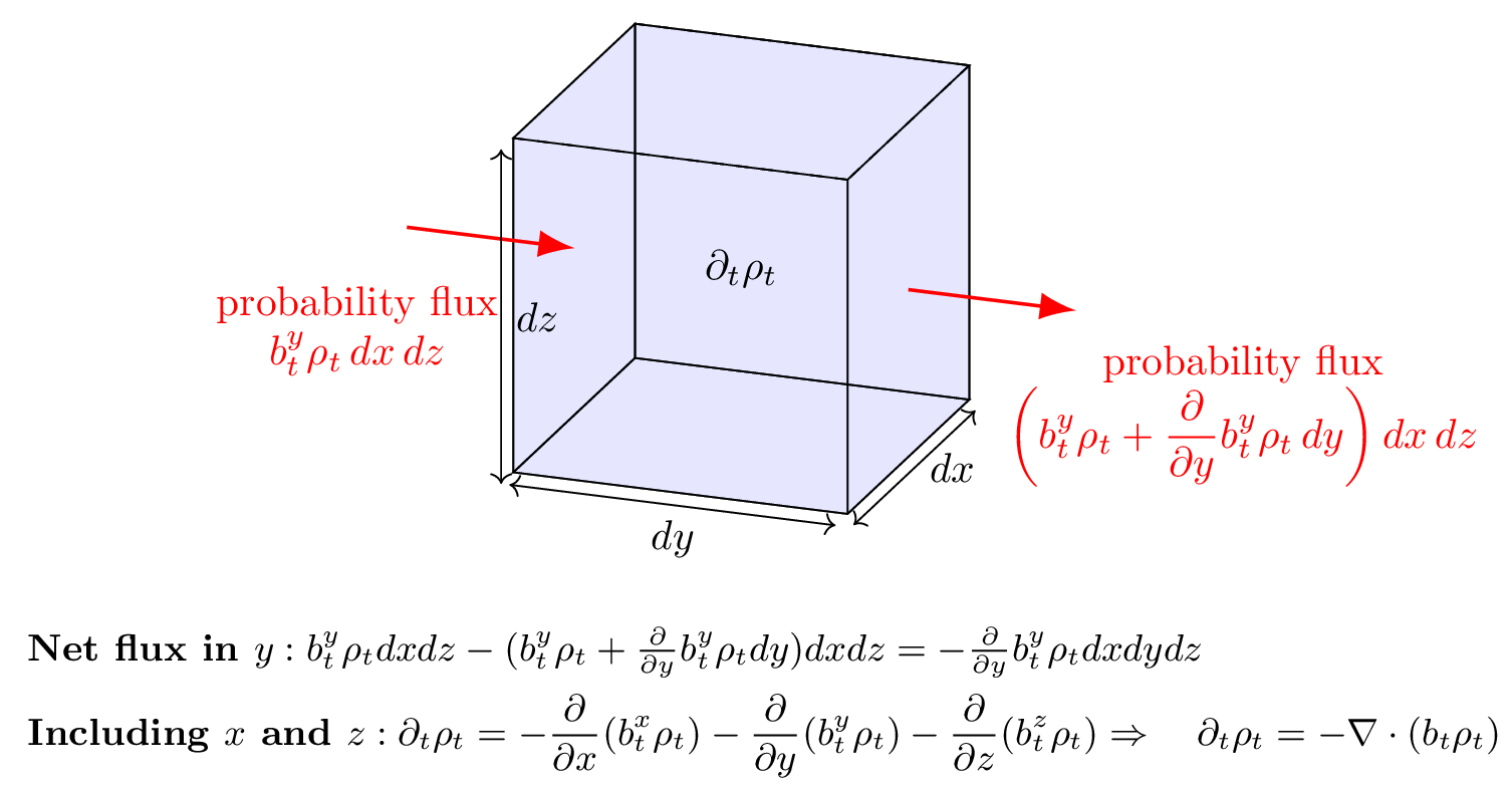— Figure 3:Intuitive derivation of the continuity equation: an incremental volume element (the cube) through which fluid flows primarily in the ( y )-direction, used to elucidate the continuity equation $\partial_t \rho_t + \nabla \cdot (b_t \rho_t) = 0$ . The incoming and outgoing probability fluxes across the $y$ -faces of the cube are represented by the red arrows, labeled with the probability fluxes $b_t^y \rho_t dx dz$ and $(b_t^y \rho_t + \left( \frac{\partial}{\partial y} b_t^y \rho_t \right) dy) dx dz$ . The net change in density within the cube ( $\partial_t \rho_t$ ) is due to the net flux in the $y$ -direction. Similar contributions from the $x$ - and $z$ -directions lead to the divergence term $\nabla \cdot (b_t \rho_t)$ . This balance ensures mass conservation in the fluid flow, as expressed by the continuity equation.

Let’s consider motion only in the $\hat y$ direction as per the figure. By dimensional analysis we can conclude that the incremental flux of probability entering the incremental volume element through the $(x,z)$ plane is given by $b_t^{y} \rho_t dx dz$ , where the superscript is used to label the velocity in the $\hat y$ direction. This flux may change at an incremental element $dy$ farther along in space, which we can estimate through taylor expansion as:

\rho_t(x + d\hat y)b_t(x + d\hat y) \approx \rho_t b_t^y + \frac{\partial}{\partial y}(\rho_t b_t^y) dy + \frac{1}{2!} \cancel{\frac{\partial^2}{\partial y^2}(\rho_t b_t^y)(dy)^2} + ...

(1)

where we only keep the first order term. Since the term on the RHS is the net flux out of the incremental volume, we can conclude that the change in probability mass at any time due to flow in the $\hat y$ direction reads as $-\partial_y b_t^y \rho_t dx dy dz$ . The same holds for flux in the $\hat x$ and $\hat z$ directions. Writing this out explicitly as the time derivative of the probability density, we have

\begin{align} &\partial_t \rho_t + \partial_x (\rho_t b_t^x) + \partial_y (\rho_t b_t^y) + \partial_z (\rho_t b_t^z) = 0 \\ & \boxed{\partial_t \rho_t + \nabla \cdot(b_t \rho_t) = 0 \quad \rho_{t=0} = \rho_0}. \end{align}

(2)

This is the continuity equation for the density $\rho_t$ and the velocity field $b_t$ , where we have included the initial condition that at time $t=0$ , we start from our base distribution $\rho_0$ . This equation is essential an equation of probability mass conservation. If we want to find a map between $\rho_0$ and $\rho_1$ , then the time dependent density $\rho_t$ arising from our map must solve (2). How do we find such a $b_t$ and $\rho_t$ to perform the transport? Eyeballing (2), things don’t look great as this is a partial differential equation (PDE). Thankfully, there is a handy trick that goes by the method of characteristics which will allow us to instead solve a family of ordinary differential equations (ODEs) that are much easier to work with. We will apply it to state the following proposition, borrowing from how it is stated in Albergo & Vanden-Eijnden (2024):

Here, we introduced the probability flow ODE, whose solutions give us characteristic curves along which we can solve (2) and produce samples $x_t \sim \rho_t$ . In particular, solving the probability flow ODE up to time $t=1$ will give us our map $X_{t=1}(x_0) = T(x_0) = x_1$ to draw samples from $\rho_1$ . The proof, which elucidates this point, is given in the dropdown bar below.

Proof 1

We want to solve the PDE:

\begin{align} \partial_t \rho_t + \nabla \cdot (b_t \rho_t) = 0 \quad \rho_{t=0} = \rho_0 \end{align}

(5)

for $\rho_t$ . To do this, we want to find characteristic curves $X_t(x)$ , with $X_{t=0}(x) = x$ along which the total derivative of $\rho_t$ w.r.t $t$ can be computed with known quantities and no other derivatives, thereby reducing the PDE, which we don’t know how to solve, into an ODE, which we do!

Taking the totaly derivative of $\rho_t(X_t(x))$ , we have using the chain rule

\begin{align} \frac{d}{dt} \rho_t(X_t(x)) = \partial_t \rho_t(X_t(x)) + {\color{blue} \nabla \rho_t(X_t(x))\cdot \dot X_t(x)}, \end{align}

(6)

where we have intentionally color-coded some terms. Next, note that we can expand the divergence term in (2) so that

\begin{align} \partial_t \rho_t + {\color{blue} b_t \cdot \nabla \rho_t} = - \nabla \cdot b_t \rho_t. \end{align}

(7)

Terms in blue are terms with $\nabla \rho_t$ that we’d like to simplify. Where does the probability flow ODE come in? If we deliberately choose $\dot X_t(x) = b_t(X_t(x))$ with appropriate initial condition $X_{t=0}(x) = x$ , then we have that $\nabla \rho_t \cdot b_t = \nabla \rho_t \cdot \dot X_t$ . Using this fact and (7) we can write

\begin{align} \frac{d}{dt} \rho_t(X_t(x)) = - \cancel{b_t(X_t(x))\cdot \nabla \rho_t(X_t(x))} - &\rho_t(X_t(x)) \nabla\cdot b_t(X_t(x)) \\ + &\cancel{\nabla \rho_t(X_x(x)) \cdot b_t(X_t(x))} \\ \end{align}

(8)

so that

\begin{align} \frac{d}{dt} \rho_t(X_t(x)) = - \rho_t(X_t(x)) \nabla\cdot b_t(X_t(x)). \end{align}

(9)

This is an ODE to describe the evolution of $\rho_t$ along curves $X_t$ , which can be solved straightfowardly as follows.

We can treat $\rho_t(X_t(x)) = \phi(t)$ only as a function of time because along the chracteristic curve, x is fixed as an initial condition. Then we have

\begin{align} \frac{d}{dt} \phi(t) = - \phi(t) \nabla \cdot b_t(X_t(x)). \end{align}

(10)

Dividing by $\phi(t)$ and integrating both sides gives

\begin{align} \int_0^t \frac{\phi'(s)}{\phi(s)} ds = - \int_0^t \nabla \cdot b_s(X_s(x)) ds \\ \log \phi(t) = \log \phi(0) - \int_0^t \nabla \cdot b_s(X_s(x)) ds \\ \phi(t) = \phi(0)e^{-\int_0^t \nabla \cdot b_s(X_s(x)) ds}, \end{align}

(11)

where we can conclude

\begin{align} \rho_t(X_t(x)) = \rho_0(x) e^{-\int_0^t \nabla \cdot b_s(X_s(x)) ds} \end{align}

(12)

Below, we visualize in Figure 4 solutions to the probability flow ODE to map out the characteristic curves $X_t$ as it goes fom $X_0$ to $X_1$ for various initial conditions.

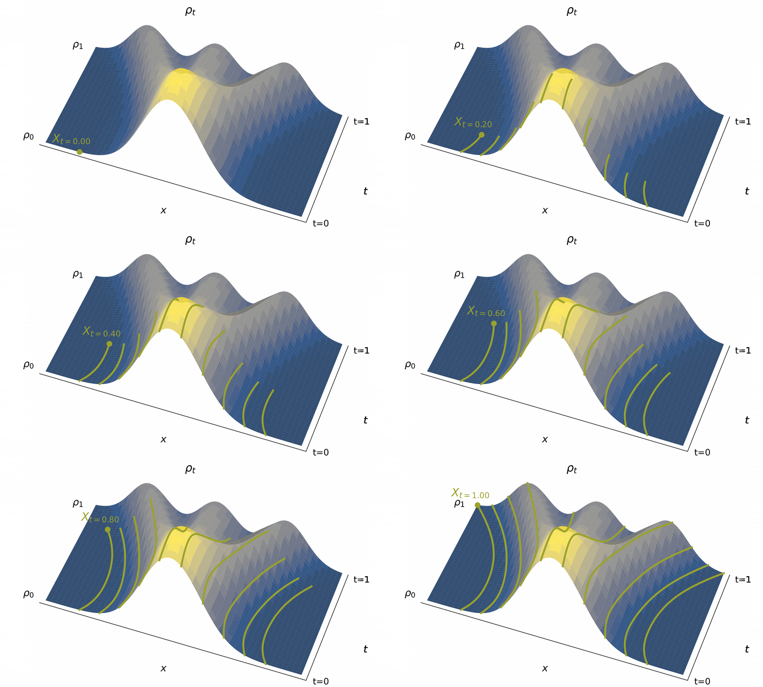
The time evolution of the density \rho_t, typified by characteristic curves X_t (used to define solutions to ) giving us the trajectories of individual particle beginning from their initial conditions. Importantly, the map — Figure 4:The time evolution of the density $\rho_t$ , typified by characteristic curves $X_t$ (used to define solutions to (2)) giving us the trajectories of individual particle beginning from their initial conditions. Importantly, the map

For a fixed $\rho_t$ , we may not know what this $b_t$ is that we need in order to solve the probability flow ODE. In fact, we don’t know it for just about all non-trivial transport problems (except for e.g. Gaussian mixtures)! How can we go about discovering one? Below we’ll implement a learning algorithm to discover what it is that is known as stochastic interpolants or flow matching (Albergo & Vanden-Eijnden (2022), Lipman et al. (2022), Liu et al. (2022)).

Stochastic Interpolants / Flow Matching¶

As we have said above, our learning problem is: given sample $x_1 \sim \rho_1$ and a base distribution with density $\rho_0$ , learn a model to generate samples $\rho_1$ . We just spent a lot of time analyzing solutions to the continuity equation involving the time dependent density $\rho_t$ and the velocity field $b_t$ to endow a flow map $X_t$ . To learn a map, I need to find a $b_t$ which solves the transport. But there’s also another problem: many such maps $X_t$ exist which meet the criteria that $X_1(x) = x_1 \sim \rho_1$ , depending on the $\rho_t$ you choose, and we haven’t discussed how to choose a $\rho_t$ !

What you’ll define below is a way to do this using the method of stochastic interpolants, which gives us a way to simultaneously choose a time dependent density $\rho_t(x)$ and learn the $b$ over a parametric function class (neural networks) that performs the associated mapping.

Let’s lay out the steps to do this in code. Here’s what we’ll need:

a python package that allows us to perform optimization over our parametric functions using autodifferentiation: PyTorch
A way to define and sample under the probability densities $\rho_0$ and $\rho_1$
A neural network that we will use as our model of the velocity field $\hat b_t(x)$
An implementation of the stochastic interpolant and the associated optimization loop used in conjunction with it to fit $\hat b_t(x)$ to the true $b_t(x)$ .
Some visualizations of the results!

We will do this on a toy dataset that defines a distribution in 2-dimensions. Let’s begin!

Software pre-requisites¶

try:
    import numpy as np
    import matplotlib.pyplot as plt
    import torch  # 2.0 or greater
    from torch.func import vmap
    
    print("All packages are installed!")
except ImportError as e:
    print(f"An error occurred: {e}. Please make sure all required packages are installed.")

    
from typing import Callable
import math

All packages are installed!

def grab(var):
    return var.detach().cpu().numpy()

device = 'cuda' if torch.cuda.is_available() else 'cpu'
print(torch.cuda.is_available())
print(device)

True
cuda

Defining and sampling our two distributions¶

To learn a generative model to sample under $\rho_1$ , we first need to define what distribution we want to sample from and what distribution we start from!

Let’s say that our data is in $\mathbb R^2$ . We will take $\rho_0$ as a Normal distribution with mean vector $\mu = (0,0)$ and identity covariance $\Sigma = I$ so that $\rho_0 \equiv \mathsf N(0, I)$ .

import torch
from torch.distributions import MultivariateNormal

class BaseDistribution:
    def __init__(self, mean, cov):
        self.mean = mean
        self.covariance = cov
        self.distribution = MultivariateNormal(mean, cov)
    
    def sample(self, n=1):
        """
        Draws $n$ samples from the Gaussian distribution.   
        """
        return self.distribution.sample((n,))
    
    def log_prob(self, x):
        """
        Evaluates the log probability of given samples $x$ under the distribution. 
        """
        return self.distribution.log_prob(x)

mean = torch.tensor([0.0, 0.0]).to(device)  # \mu \in R^2
cov = torch.tensor([[1.0, 0.0], [0.0, 1.0]]).to(device)  # \Sigma \in R^{2x2}

base = BaseDistribution(mean, cov)

Let’s choose our target distribution to be: a checkerboard in in 2d space or a Gaussian Mixture defined as follows:¶

## checker
# ndim = 2
# def target(bs):
#     x1 = torch.rand(bs) * 4 - 2
#     x2_ = torch.rand(bs) - torch.randint(2, (bs,)) * 2
#     x2 = x2_ + (torch.floor(x1) % 2)
#     return (torch.cat([x1[:, None], x2[:, None]], 1) * 2)


from torch.distributions.mixture_same_family import MixtureSameFamily
from torch.distributions.normal import Normal
from torch.distributions.categorical import Categorical
from torch.distributions.independent import Independent
from torch.distributions.multivariate_normal import  MultivariateNormal




class Prior(torch.nn.Module):
    """
    Abstract class for prior distributions of normalizing flows. The interface
    is similar to `torch.distributions.distribution.Distribution`, but batching
    is treated differently. Parameters passed to constructors are never batched,
    but are aware of the target (single) sample shape. The `forward` method then
    accepts just the batch size and produces a batch of samples of the known
    shape.
    """
    def forward(self, batch_size):
        raise NotImplementedError()
    def log_prob(self, x):
        raise NotImplementedError()
    def draw(self, batch_size):
        """Alias of `forward` to allow explicit calls."""
        return self.forward(batch_size)
    

    
class GMM(Prior):
    def __init__(self, loc=None, var=None, scale = 1.0, ndim = None, nmix= None, device=device, requires_grad=False):
        super().__init__()
        
        self.device = device
        self.scale = scale       ### only specify if loc is None
        def _compute_mu(ndim):
                return self.scale*torch.randn((1,ndim))
                        
        if loc is None:
            self.nmix = nmix
            self.ndim = ndim 
            loc = torch.cat([_compute_mu(ndim) for i in range(1, self.nmix + 1)], dim=0)
            var = torch.stack([1.0*torch.ones((ndim,)) for i in range(nmix)])
        else:
            self.nmix = loc.shape[0]
            self.ndim = loc.shape[1] ### locs should have shape [n_mix, ndim]
            
        self.loc = loc   ### locs should have shape [n_mix, ndim]
        self.var = var   ### should have shape [n_mix, ndim]
        
        if requires_grad:
            self.loc.requires_grad_()
            self.var.requires_grad_()
        
        mix = Categorical(torch.ones(self.nmix,).to(device))
        comp = Independent(Normal(
                     self.loc, self.var), 1)
        self.dist = MixtureSameFamily(mix, comp)
        
    def log_prob(self, x):
        logp = self.dist.log_prob(x)
        return logp
    
    
    def forward(self, batch_size):
        x = self.dist.sample((batch_size,))
        return x
    
    def rsample(self, batch_size):
        x = self.dist.rsample((batch_size,))
        return x
    
nmix = 8
ndim = 2
def _compute_mu(i):
            return 5.0 * torch.Tensor([[
                        torch.tensor(i * math.pi / 4).sin(),
                        torch.tensor(i * math.pi / 4).cos()]]).to(device)
mus_target = torch.stack([_compute_mu(i) for i in range(nmix)]).squeeze(1).to(device)
var_target = torch.stack([torch.tensor([0.7, 0.7]) for i in range(nmix)]).to(device)


target = GMM(mus_target, var_target)
target_samples  = target(10000)

Below we can visualize both of the distributions by drawing samples from them and plotting them

bs = 5000
c = '#62508f' # plot color

x0s = grab(base.sample(bs))
x1s = grab(target(bs))

fig, (ax0, ax1) = plt.subplots(nrows=1, ncols=2, figsize=(10,5))

ax0.scatter(x0s[:,0], x0s[:,1], alpha = 0.5, c = c);
ax0.set_xlim(-4,4), ax0.set_ylim(-4,4)
ax0.set_title(r"Samples under $\rho_0$", fontsize = 16)
ax0.set_xticks([-4,0,4]), ax0.set_yticks([-4,0,4])

ax1.scatter(x1s[:,0], x1s[:,1], alpha = 0.5, c = c);
ax1.set_xlim(-8,8), ax1.set_ylim(-8,8)
ax1.set_title(r"Samples under $\rho_1$", fontsize = 16)
ax1.set_xticks([-4,0,4]), ax1.set_yticks([-4,0,4]);
plt.show();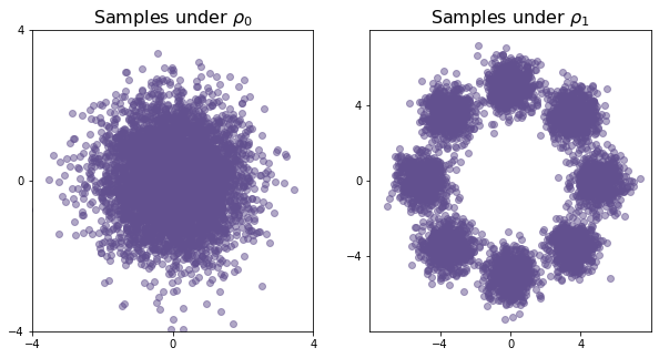

Building a map between $\rho_0$ and $\rho_1$ with the interpolant¶

You have been learning in class that you can use the method of stochastic interpolants to define a time dependent density $\rho_t(x)$ that connects $\rho_0$ to $\rho_1$ and allows us to learn the associated velocity field $b_t(x)$ that would map samples from one to samples from another.

Let’s introduce the interpolant function here and make some statements about it. The stochastic interpolant $I_t$ is a stochastic process given as:

I_t = \alpha_t x_0 + \beta_t x_1 \quad \text{where} x_0 \sim \rho_0 \text{ and } x_1 \sim \rho_1

(13)

When $x_0, x_1$ are drawn accordingly, we say that the stochastic interpolant $I_t$ is a sample under the time dependent density i.e. $I_t \sim \rho_t(x)$ .
The velocity field associated to this $\rho_t(x)$ is given by the conditional expectation of the time dynamics of the interpolant, namely:

b_t(x) = \mathbb E[ \dot I_t | I_t = x]

(14)

What do we mean when we say $I_t$ samples $\rho_t(x)$ ? Well let’s take a look by implementing it. We will make a class called Interpolant that implements $I_t$ and its time derivative.

Proof 2

The interpolant has probability density given by

\rho_t(x) = \int_{\mathbb R^{d\times d}} \delta(x - I_t(x_0, x_1))\rho(x_0, x_1) dx_0 dx_1

(15)

Taking the derivative of (15) and using the chain rule on the right-hand side, we see that

\begin{align} \partial_t \rho_t &= - \int \dot I_t \cdot \nabla \delta (x - I_t) \rho(x_0, x_1) dx_0 dx_1\\ &= -\nabla \cdot \int \dot I_t \delta (x - I_t) \rho(x_0, x_1) dx_0 dx_1 = - \nabla \cdot j_t \end{align}

(16)

for some probability current $j_t = b_t \rho_t$ which completes the continuity equation given in (2). Dividing by $\rho_t$ to isolate $b_t$ we see that

\begin{align} b_t = \frac{\int \dot I_t \delta (x - I_t) \rho(x_0, x_1)}{\int\delta (x - I_t) \rho(x_0, x_1)} = \mathbb E[ \dot I_t | I_t = x] \end{align}

(17)

## using alpha(t) = (1-t) and beta(t) = t
class Interpolant:
    def alpha(self, t):
        return 1.0 - t
    
    def dotalpha(self, t):
        return -1.0 + 0*t
    
    def beta(self, t):
        return t
    
    def dotbeta(self, t):
        return 1.0 + 0*t
    
    def _single_xt(self, x0, x1, t):
        return self.alpha(t)*x0 + self.beta(t)*x1
    
    def _single_dtxt(self, x0, x1, t):
        return self.dotalpha(t)*x0 + self.dotbeta(t)*x1
    
    def xt(self, x0, x1, t):
        return vmap(self._single_xt, in_dims=(0, 0, 0))(x0,x1,t)
    
    def dtxt(self, x0, x1, t):
        return vmap(self._single_dtxt, in_dims=(0, 0, 0))(x0,x1,t)
    
    
interpolant = Interpolant()

bs  = 10000
x0s = base.sample(bs).to(device)
x1s = target(bs).to(device)
t   = 0.2*torch.ones(bs).to(device)

xts = interpolant.xt(x0s, x1s, t)

In the above code, we implement the interpolant for a single sample of $x_0$ , $x_1$ , and $t$ , which have shape [d], [d], [1] respectively. Then, we use a tool in pytorch called vmap which allows us to generalize the code for arbitrary batches of samples of $x_0, x_1$ and $t$ . That way, if I have $N$ samples of $x_0$ , $x_1$ and $t$ , I can compute the interpolant for all $N$ of them at once using vmap.

This means I can feed the function interpolant.xt a batch of samples of shape [N, d] for $x_0$ and $x_1$ and of shape [N] for time.

Let’s see what happens when I sample $\rho_t(x)$ at various times along $[0,1]$ :

bs = 8000
ncol = 6
ts   = torch.linspace(0, 1, ncol)
c = '#62508f'

fig, axes = plt.subplots(1, ncol, figsize=(ncol*4,4))

for i, t in enumerate(ts):
    
    
    tt  = t.repeat(bs).to(device)
    x0s = base.sample(bs).to(device)
    x1s = target(bs).to(device)
    xts = interpolant.xt(x0s, x1s, tt)
    
    axes[i].scatter(grab(xts[:,0]), grab(xts[:,1]), alpha = 0.08, c = c); # plot samples x_t \sim \rho_t
    
    axes[i].set_xticks([])
    axes[i].set_title(r'$\rho(t = %.1f)$' % t, fontsize = 20, weight='bold')
    axes[i].set_xlim(-8,8)
    axes[i].set_ylim(-8,8)
    
    if i !=0:
        axes[i].set_yticks([])

plt.show();

Neural Network $\hat b_t(x)$ to model $b_t(x)$ ¶

Now we need to define a neural network which has learnable parameters to model $b_t(x)$ . Recall that the velocity field takes in a time coordinate and a spatial sample which is $\mathbb R^2$ . This means that our neural network approximation $\hat b_t(x)$ should be a function that has an input size of $1 + \text{space dim} = 3$ and should have an output dimension of $\text{space dim} = 2$ .

To define a neural network, we’ll use PyTorch’s torch.nn.Module library which allows us to compose parts of the neural network in a way that allows us to take derivatives with respect to the networks weights:

from torch.func import jacrev, grad

class VelocityField(torch.nn.Module):
    # a neural network that takes x in R^d and t in [0, 1] and outputs a a value in R^d
    def __init__(self, d,  hidden_sizes = [256, 256], activation=torch.nn.ReLU):
        super(VelocityField, self).__init__()
        
        layers = []
        prev_dim = d + 1  #
        for hidden_size in hidden_sizes:
            layers.append(torch.nn.Linear(prev_dim, hidden_size))
            layers.append(activation())
            prev_dim = hidden_size  # Update last_dim for the next layer

        # final layer
        layers.append(torch.nn.Linear(prev_dim, d))
        
        # Wrap all layers in a Sequential module
        self.net = torch.nn.Sequential(*layers)
    
    def _single_forward(self, x, t):  
        t = t.unsqueeze(-1)
        return self.net(torch.cat((x, t)))
    
    def forward(self, x, t):
        return vmap(self._single_forward, in_dims=(0,0), out_dims=(0))(x,t)

Let’s check to make sure our neural network class works by making some fake data and seeing that it outputs something of the right shape

d = 2
b =  VelocityField(d, hidden_sizes=[512, 512, 512]).to(device)


bs = 10 ## simple test batch size
x = torch.rand(bs, d).to(device)
t = torch.rand(bs).to(device)
print(x.shape)
print(t.shape)
out = b.forward(x,t) ## should output something of shape [bs, d]

torch.Size([10, 2])
torch.Size([10])

Loss function and learning¶

Now that we have a suitable neural network to optimize, we need to specify the learning rule to update the weights of $\hat b_t(x)$ .

Given that the velocity field of the interpolant is $b_t(x) = \mathbb E [ \dot I_t | I_t = x]$ , it should be the unique minimizer of the least squares loss given by:

\mathcal L[\hat b] = \int_0^1 \mathbb E| \hat b(t,I_t) - \dot I_t|^2 dt

(18)

where expectation is taken over $(x_0, x_1) \sim \rho(x_0, x_1)$ .

Let’s go ahead and implement this in code:

def _single_loss(b, interpolant, x0, x1, t):
    """
    Interpolant loss function for a single datapoint of (x0, x1, t).
    """
    It   = interpolant._single_xt(  x0, x1, t)
    dtIt = interpolant._single_dtxt(x0, x1, t)
    
    bt          = b._single_forward(It, t)
    loss        = 0.5*torch.sum(bt**2) - torch.sum((dtIt) * bt)
    return loss


loss_fn = vmap(_single_loss, in_dims=(None, None, 0, 0, 0), out_dims=(0), randomness='different')

N = 10
x0s = base.sample(N).to(device)
x1s = target(N).to(device)
ts  = torch.rand(N).to(device)
loss_fn(b, interpolant, x0s, x1s, ts).mean()

tensor(0.2853, device='cuda:0', grad_fn=<MeanBackward0>)

Training step¶

Now that we have constructed our loss, let’s put it in a loop to interatively update the parameters of $\hat b$ as we move toward the minimizer of $\mathcal L[\hat b]$ .

To perform this parameter update, we need to introduce a pytorch optimizer that performs the gradient update for us. We do that via the following, specifying a learning rate lr. We use the Adam optimizer, which is a fancier version of SGD.

lrb = 2e-3 ## learning rate
opt = torch.optim.Adam([
    {'params': b.parameters(), 'lr': lrb} ])
sched = torch.optim.lr_scheduler.StepLR(opt, step_size=1500, gamma=0.6)

Now lets use it in a function called train_step which will perform our iteration:

def train_step(b, interpolant, opt, sched, N):
    
    ## draw N samples form each distribtuion and from time uniformly
    x0s = base.sample(N).to(device)
    x1s = target(N).to(device)
    ts  = torch.rand(N).to(device)
    
    # evaluate loss 
    loss_val = loss_fn(b, interpolant, x0s, x1s, ts).mean()
    
    # perform backprop
    loss_val.backward()
    opt.step()
    sched.step()
    opt.zero_grad()
    
    res = {
            'loss': loss_val.detach(),
        }
    return res

Running the Training¶

We are now ready to train our model. Let’s build a loop that runs for n_opt stepsand store the loss over time.

n_opt = 5000
bs    = 2500

losses = []
from tqdm import tqdm
pbar = tqdm(range(n_opt))
for i in pbar:
    
    res = train_step(b, interpolant, opt, sched, bs)
    loss = grab(res['loss'])
    
    losses.append(loss)
    pbar.set_description(f'Loss: {loss:.4f}')

Loss: -8.8316: 100%|██████████| 5000/5000 [00:13<00:00, 362.18it/s]

plt.plot(losses);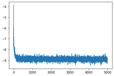

Implementing the ODE integrator¶

Now that we’ve learned $b_t(x)$ , we can use it in the probability flow ODE

\dot X_t(x) = b_t(X_t(x))

(19)

to get our generative model. To solve this ODE, we will use the Euler method, and iterate on the procedure:

X_{t + \Delta t} = X_t + \Delta t \, b_t(X_t), \qquad X_{t=0} \sim \rho_0, \qquad

(20)

We will do this with the following class called ODEIntegrator which implements the iterative step and performs the rollout over the interval $t \in [0,1]$ .


class ODE:
    def __init__(self, b, interpolant, n_step):
        
        self.b           = b
        self.interpolant = interpolant
        self.n_step      = n_step
        self.ts          = torch.linspace(0.0,1.0, n_step + 1).to(device)
        self.dt          = self.ts[1] - self.ts[0]
    
    
    
    def step(self, x, t):
        return x + self.b(x, t)*self.dt 
    
    def solve(self, x_init):
        
        bs = x_init.shape[0]
        xs = torch.zeros((self.n_step, *x_init.shape))
        x = x_init
        for i,t in enumerate(self.ts[:-1]):
            t = t.repeat(len(x))
            x = self.step(x,t)
            xs[i] = x
        return xs
    
    
ode  = ODE(b, interpolant, n_step = 80)


x_init = base.sample(20000).to(device)
xfs    = ode.solve(x_init)
x1s = grab(xfs[-1])

Implementing the SDE integrator¶

We can also use the velocity field $b_t(x)$ in the generative model based on the SDE

dX_t(x) = b(t,X_t(x)) + \epsilon_t s_t(X_t)dt + \sqrt{2\epsilon_t} dW_t

(21)

where $s_t(x)$ is the score and $\epsilon_t\ge 0$ is the diffusion coefficient. To get $s_t(x)$ we can use its relation to $b_t(x)$ :

s_t(x) = \frac{\beta_t b_t(x)-\dot\beta_t x}{\alpha_t(\alpha_t\dot\beta_t-\dot\alpha\beta_t)}

(22)

Since $\alpha_1 =0$ , to avoid problems near $t=1$ , below we will use $\epsilon_t = \epsilon \alpha_t$ for some constant $\epsilon >0$ , and calculate directly $\alpha_t s_t(x)$ instead of $s_t(x)$ .

To solve the SDE, we will use the Euler-Maruyama method, and iterate on the procedure:

X_{t + \Delta t} = X_t + \Delta t \, b_t(X_t) + \Delta t \, \epsilon_t s_t(X_t) + \sqrt{2\epsilon_t\Delta t}\, \xi_t, \qquad x_{t=0} \sim \rho_0, \qquad

(23)

where $\xi_t\sim N(0,\text{Id})$ .

We will do this with the following class called SDEIntegrator which implements the iterative step and performs the rollout over the interval $t \in [0,1]$ .

class SDE:
    def __init__(self, b, interpolant, eps, n_step):
        
        self.b           = b
        self.interpolant = interpolant
        self.n_step      = n_step
        self.ts          = torch.linspace(0.0,0.99, n_step + 1).to(device)
        self.dt          = self.ts[1] - self.ts[0]
        self.eps         = eps.to(device)
        self.sqrtepsdt   = torch.sqrt(torch.tensor(2.0)*self.eps*self.dt).to(device)
  
    def alphascore(self, x, t):
        alpha = self.interpolant.alpha(t).unsqueeze(-1)
        dotalpha = self.interpolant.dotalpha(t).unsqueeze(-1)
        beta = self.interpolant.beta(t).unsqueeze(-1)
        dotbeta = self.interpolant.dotbeta(t).unsqueeze(-1)
        

        return (beta*self.b(x, t)-dotbeta*x)/(alpha*dotbeta-dotalpha*beta)
    
    def step(self, x, t):
        alpha = self.interpolant.alpha(t).unsqueeze(-1)
        return x + (self.b(x, t)+self.eps*self.alphascore(x, t))*self.dt + self.sqrtepsdt*torch.sqrt(alpha)*torch.randn(x.size()).to(device)
    
    def solve(self, x_init):
        
        bs = x_init.shape[0]
        xs = torch.zeros((self.n_step, *x_init.shape))
        x = x_init
        for i,t in enumerate(self.ts[:-1]):
            t = t.repeat(len(x))
            x = self.step(x,t)
            xs[i] = x
        return xs
    
    
sde  = SDE(b, interpolant, eps = torch.tensor(2.0), n_step = 80)


# x_init = base.sample(20000)
xf2s    = sde.solve(x_init).to(device)
x2s = grab(xf2s[-1])

Now let’s plot the results of our generative models:

c = '#62508f' # plot color
fig, axes = plt.subplots(1,2, figsize=(10,5))
axes[0].scatter(x1s[:,0], x1s[:,1], alpha = 0.03, c = c)
axes[0].set_title(r"Samples from the prob. flow ODE", fontsize = 18)
axes[0].set_xticks([-4,0,4]), axes[0].set_yticks([-4,0,4]);

axes[1].scatter(x2s[:,0], x2s[:,1], alpha = 0.03, c = c)
axes[1].set_title(r"Samples from the SDE", fontsize = 18)
axes[1].set_xticks([-4,0,4]), axes[1].set_yticks([-4,0,4]);

plt.tight_layout();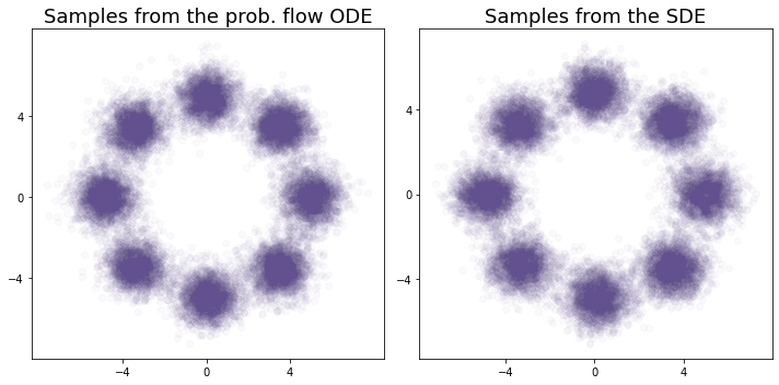

What’s next?¶

Now that we’ve built out the machinery for learning a dynamical generative model for a simple 2D distribution, we can turn to ask about image generation, which for coding purposes just means replacing our feed forward neural network with a much better one (that we’ll see on the next page), and loading a different data source. Let’s proceeed to that.